Create Pivot Table Report in Microsoft Excel

1. Create a report containing the fields you'd like to create a PivotTable on. For example, say you want to analyze sales by country and product. Create a new report and select Country from the Customers table, Product Name from the Products table, and Total Price from the Order Details table.

2. Set any desired filter for the report.

3. Output the report to a Microsoft Excel - Data Only file by going to Output page in the Reports Explorer, choosing File for the Output to option, clicking the File button, choosing Microsoft Excel - Data Only (*.xls) in the Save as type option, entering the name of the file to create, and clicking Save. Click the Process button to create the file.

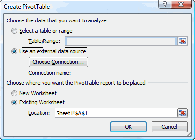
4. Start Microsoft Excel and create a new document. From the Insert tab of the ribbon, choose PivotTable. In the Create PivotTable dialog, select Use an external data source, then click the Choose Connection button.

5. In the Existing Connections dialog, click the Browse for More button. In the Select Data Source dialog, select the directory where you told Student Manager Reports to create the Excel file and select the file. Click Open.

6. In the Select Table dialog, click OK. Click OK in the Create PivotTable dialog.

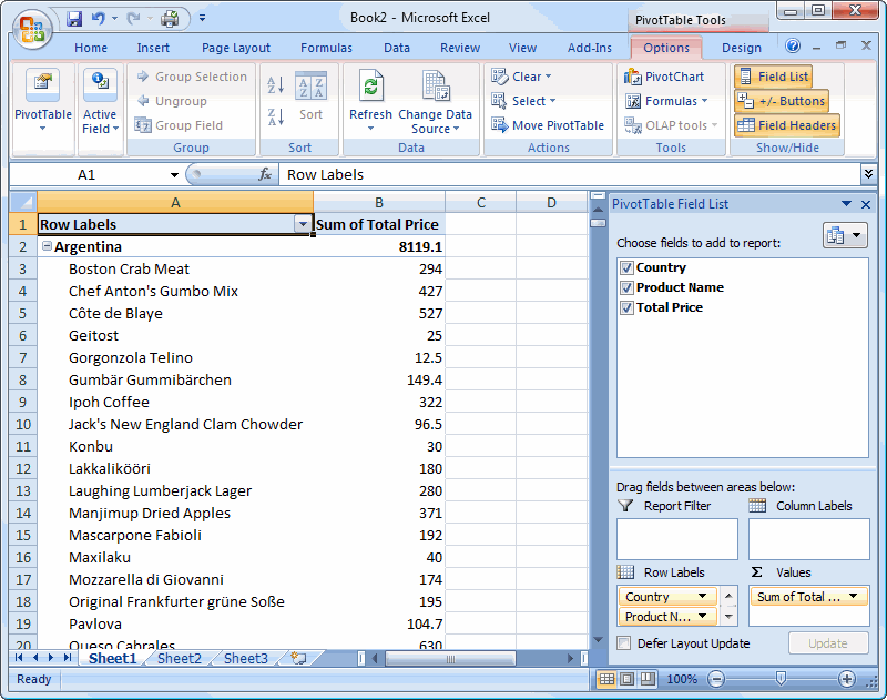
7. In the Pivot Table List, turn on the fields you want included in the PivotTable.

8. Excel immediately creates a PivotTable for you. Format the PivotTable, filter certain values out of the rows or columns, print the table, save it, etc.